

Nitrogen-Phytoplankton-Salinity MATLAB Example
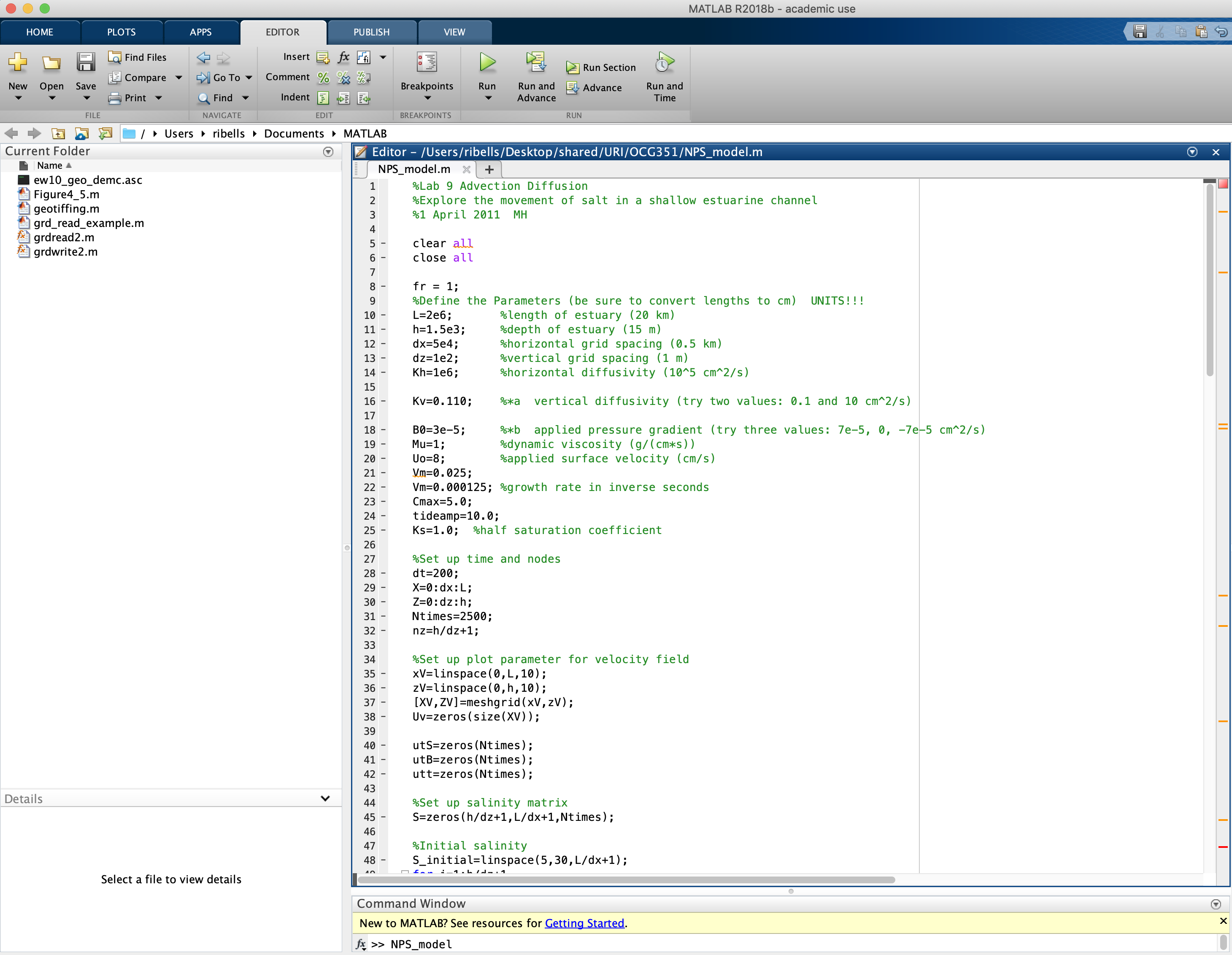
MATLAB is a popular script-driven computing environment for doing ocean science data analysis. Below is an example of a MATLAB script, using a Nitrogen-Phytoplankton-Salinity (NPS) model as an example. Compare the MATLAB script with the Python script to see the differences in approach. The MATLAB script is shown here:
%Advection Diffusion Lab
%Explore the movement of salt in a shallow estuarine channel
%1 April 2011  MH

clear all
close all

fr = 1;
%Define the Parameters (be sure to convert lengths to cm)  UNITS!!!
L=2e6;       %length of estuary (20 km)
h=1.5e3;     %depth of estuary (15 m)
dx=5e4;      %horizontal grid spacing (0.5 km)
dz=1e2;      %vertical grid spacing (1 m)
Kh=1e6;      %horizontal diffusivity (10^5 cm^2/s)

Kv=0.110;    %*a  vertical diffusivity (try two values: 0.1 and 10 cm^2/s)

B0=3e-5;     %*b  applied pressure gradient (try three values: 7e-5, 0, -7e-5 cm^2/s)
Mu=1;        %dynamic viscosity (g/(cm*s))
Uo=8;        %applied surface velocity (cm/s)
Vm=0.025;
Vm=0.000125; %growth rate in inverse seconds
Cmax=5.0;
tideamp=10.0;
Ks=1.0;  %half saturation coefficient

%Set up time and nodes
dt=200;
X=0:dx:L;
Z=0:dz:h;
Ntimes=2500;
nz=h/dz+1;

%Set up plot parameter for velocity field
xV=linspace(0,L,10);
zV=linspace(0,h,10);
[XV,ZV]=meshgrid(xV,zV);
Uv=zeros(size(XV));

utS=zeros(Ntimes);
utB=zeros(Ntimes);
utt=zeros(Ntimes);

%Set up salinity matrix
S=zeros(h/dz+1,L/dx+1,Ntimes);

%Initial salinity
S_initial=linspace(5,30,L/dx+1);
for i=1:h/dz+1
    S(i,:,1)=S_initial;
end

%Boundary Conditions
S(:,1,:)=5;
S(:,L/dx+1,:)=30;

%Initial concentration
C_initial=linspace(Cmax,0,L/dx+1);
P_initial=linspace(0,0,L/dx+1);
for i=1:h/dz+1
    C(i,:,1)=C_initial;
    P(i,:,1)=P_initial;
end

%Boundary Conditions: depth, distance, time
C(:,1,:)=Cmax;
C(:,L/dx+1,:)=0;
P(:,1,:)=0;
P(1:6,L/dx+1,:)=5;
P(7:h/dz+1,L/dx+1,:)=0;

%Calculate the average flux of a day
sumU=zeros(size(Z));
Lp3=floor((L/dx)/3);
Lp6=floor((L/dx)*2/3);

averageU=sumU/(24*3600);
xlabel('Velocity(cm/s)')
ylabel('Depth(cm)')
B=B0;
Ures=(0.5*B/Mu).*Z.^2+((Uo/h)-(0.5*B*h/Mu)).*Z;

%Calculate salinity over time
for k=2:Ntimes-800     %TIME
    %B=B0*sin(k*dt/(24*3600)*2*pi);
    utide=tideamp*sin(k*dt/(12*3600)*2*pi);
    U=Ures+utide;

    utS(k)=U(14);
    utB(k)=U(4);
    utt(k)=(k*dt)/(3600*24);

    velocityh=(0.5*B/Mu).*zV.^2+((Uo/h)-(0.5*B*h/Mu)).*zV;
    velocityh=velocityh';
    Uh=repmat(velocityh,1,10);
    C(:,1,k)=5;
    P(1:6,L/dx+1,k)=5;
    for j=2:L/dx       %LENGTH
        for i=2:h/dz   %DEPTH
            Nsrc=Vm*(C(i,j,k-1)/(Ks+Cmax))*P(i,j,k-1)*(i/(h/dz))*dt;
            if U(i)>0
                S(i,j,k)=S(i,j,k-1)-U(i)*(dt/dx)*(S(i,j+1,k-1)-S(i,j,k-1))+Kh*(dt/dx^2)*(S(i,j+1,k-1)-2*S(i,j,k-1)+S(i,j-1,k-1))+Kv*(dt/dz^2)*(S(i+1,j,k-1)-2*S(i,j,k-1)+S(i-1,j,k-1));
                C(i,j,k)=C(i,j,k-1)-U(i)*(dt/dx)*(C(i,j+1,k-1)-C(i,j,k-1))+Kh*(dt/dx^2)*(C(i,j+1,k-1)-2*C(i,j,k-1)+C(i,j-1,k-1))+Kv*(dt/dz^2)*(C(i+1,j,k-1)-2*C(i,j,k-1)+C(i-1,j,k-1));
                P(i,j,k)=P(i,j,k-1)-U(i)*(dt/dx)*(P(i,j+1,k-1)-P(i,j,k-1))+Kh*(dt/dx^2)*(P(i,j+1,k-1)-2*P(i,j,k-1)+P(i,j-1,k-1))+Kv*(dt/dz^2)*(P(i+1,j,k-1)-2*P(i,j,k-1)+P(i-1,j,k-1));
                C(i,j,k)=C(i,j,k)-Nsrc;
                if C(i,j,k) < 0.0 ;
                    C(i,j,k)=0.0;
                end
                P(i,j,k)=P(i,j,k)+Nsrc;
            else
               S(i,j,k)=S(i,j,k-1)-U(i)*(dt/dx)*(S(i,j,k-1)-S(i,j-1,k-1))+Kh*(dt/dx^2)*(S(i,j+1,k-1)-2*S(i,j,k-1)+S(i,j-1,k-1))+Kv*(dt/dz^2)*(S(i+1,j,k-1)-2*S(i,j,k-1)+S(i-1,j,k-1));
               C(i,j,k)=C(i,j,k-1)-U(i)*(dt/dx)*(C(i,j,k-1)-C(i,j-1,k-1))+Kh*(dt/dx^2)*(C(i,j+1,k-1)-2*C(i,j,k-1)+C(i,j-1,k-1))+Kv*(dt/dz^2)*(C(i+1,j,k-1)-2*C(i,j,k-1)+C(i-1,j,k-1));
               C(i,j,k)=C(i,j,k)-Nsrc;
                if C(i,j,k) < 0.0 ;
                    C(i,j,k)=0.0;
                end
               P(i,j,k)=P(i,j,k-1)-U(i)*(dt/dx)*(P(i,j,k-1)-P(i,j-1,k-1))+Kh*(dt/dx^2)*(P(i,j+1,k-1)-2*P(i,j,k-1)+P(i,j-1,k-1))+Kv*(dt/dz^2)*(P(i+1,j,k-1)-2*P(i,j,k-1)+P(i-1,j,k-1));
               P(i,j,k)=P(i,j,k)+Nsrc;
            end
        end
    end
    S(1,:,k)=S(2,:,k);  %depth, dist, time
    S(end,:,k)=S(end-1,:,k);

    for i=2:nz-1
        if U(i)>=0
            S(i,end,k)=S(i,end-1,k);
            else
            S(i,end,k)=30.0;
        end
    end

    P(1,:,k)=P(2,:,k);  %depth, dist, time
    P(end,:,k)=P(end-1,:,k);

    C(1,:,k)=C(2,:,k);
    C(end,:,k)=C(end-1,:,k);

    if (k>=100 & mod(k,60)==0)
    figure(1)
    box('on');
    hold('all');
    subplot(3,1,1)
    pcolor(S(:,:,k));
    shading interp
    caxis([0 30])
    text(30,20,['Time is ' num2str(k*dt/3600) 'hours'] );
    title('Salinity','FontSize', 18);

    subplot(3,1,2)
    pcolor(C(:,:,k));
    shading interp
    caxis([0 5])
    title('Nitrogen' ,'FontSize', 18);
    ylabel('Height above bottom,m','FontSize',11)

    subplot(3,1,3)
    pcolor(P(:,:,k));
    shading interp
    caxis([0 5])
    xlabel('Distance along West Passage,km','FontSize',11)
    title('Phytoplankton','FontSize', 18);

    pause(.01)
    M(fr) = getframe(gcf);
    fr = fr+1;

    clf('reset')
    end
end

movie2avi(M,'lab10_np','FPS',1) %make an AVI movie from timestep plots
The script runs through MATLAB application software. Open a script file (they normally have a .m extension) and click on the Run button:
With MATLAB, all loaded modules are available for use in the script. You can determine which modules load when you launch the MATLAB program.
I probably have overdone it as MATLAB takes a while to load as a result of all the modules it readies at launch time. I am only using about 2% of them in
the script. When you run a script within MATLAB, you can run one line at a time (like the control we
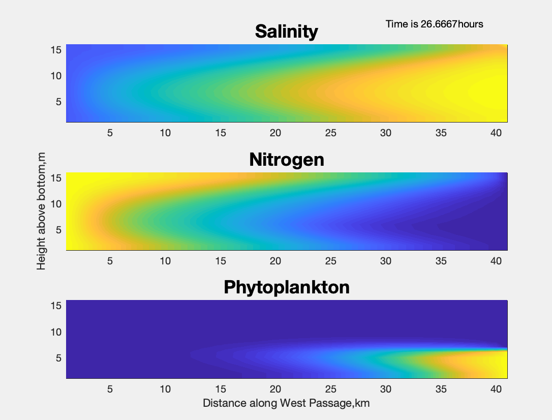
have over using Python in a Jupyter notebook). After each timestep loop in the model, a figure dialogue window shows the result.
26.67 hours into the simulation, the figure dialogue window shows:
The plotting interface in MATLAB is straight-forward and similar to the Matplotlib services interface in Python.