

Class on March 4 2019
Bruce started with an interactive whiteboard discussion of Python versus JavaScript as data visualization content languages.
Bruce emphasized the significance of the back-end processes by which data is acquired, stored, and managed. Data processing is a process by which data is thoughfully managed through meaningful transformations. As design students, the students learned they'd be held responsible for understanding relational theory as a best-practices approach to data processing. There are three roles relevant to understanding relational theory:
1. Data Modelers master techniques to coordinate data acquisition based on usefulness and contribution to a holistic view of the needs of those who will use it.
2. Data Administrators master techniques to implement and fill a data model by using hardware and software techniques to support the data warehousing.
3. Data Analysts master techniques to perform analysis on a data collection that has beejn compliant to a data model.
The demand for the three roles is skewed toward the analyst role (our role in class) since data modelers and data administrators can perform their roles once for a data collection's requirements and yet the analysis is a continuous process as new data becomes available in the collection (and with earth and ocean science data, the amount of new data becoming available through satellite, ground sensor, ship platform, remote vehicle, embedded telecommunications, etc. is constant and of great magnitude). Data administration services are performed by specialty software more and more often (reducing the need for human labor), which puts some responsibility on the data modeler to document modeling results in a format the software can understand in the absense of a data administrator.
Both the data modeler and data administrator roles are critical and usually well-compensated when performed in a large organization with data of great value. Smaller organizations might require that the same person perform two or three of the roles.
Bruce led a simple example of creating a data model for a restaurant (e.g. employee data, customer data, menu data, and a meal relationship between the three). The result was captured on a whiteboard:
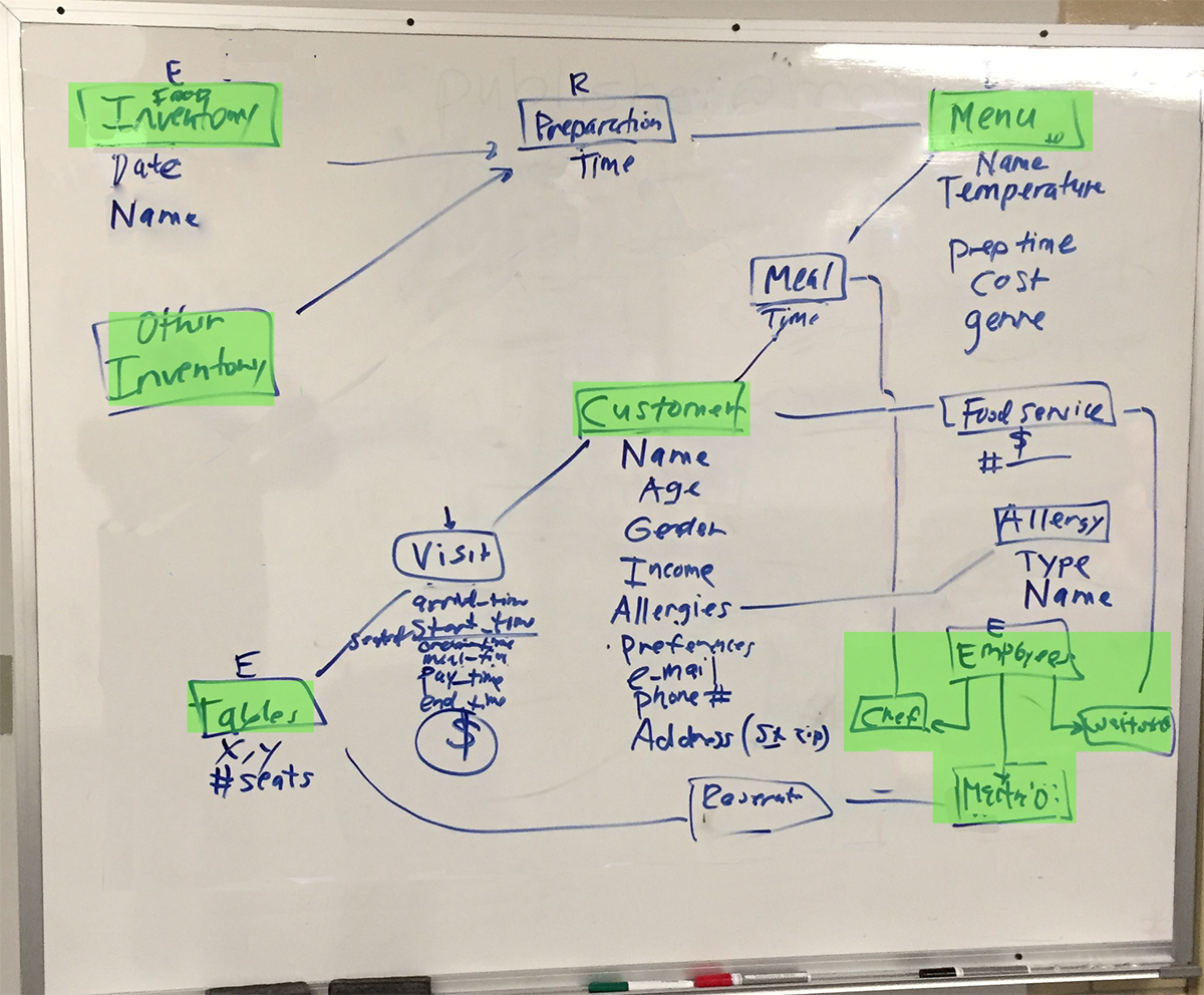
and implemented in a restaurant database exported to an SQL script file which would be used in future classes for studying SQL (Structured Query Language) query techniques.
Entities (organizational assets usually physical in nature or at least best described by a noun) discussed are highlighted in green, while relationships (other boxed items without highlighting) are identified as relating one or more entities together in some kind of actionable event (better defined by a verb more often). Important data attributes are allocated into data tables based on their value of describing an entity or describing a component of a relationship. Modeling tries to minimal the redundancy of data items to avoid update errors.
Students can implement their data model as data administrators within the class MAMP software environment. MAMP is a software package that includes key components for data administration and analysis roles:
MySQL is a relational database managment tool
Apache Server is a web server environment
MyPHPAdmin is a forms-based implementation of MySQL interaction tools
PHP is middleware for serving relational data to web server resources for serving content.
Once the restaurant database is created and the restaurant SQL command sequence is imported, students can learn from a series of SQL commands that demonstrate the usefulness of ALTER, INSERT INTO, DELETE, UPDATE, and SELECT commands.
First, let's add the waitstaff ID to each VISIT. We alter the visit table:
But, alas, she left us before ordering:
We can determine the total tips for each waitstaff:
We realize that we want to connect the customer's meal to the customer's visit:
We can return to looking at average revenue and break the analysis out by customer:
We can also add an ORDER BY clause to see the results in a particular order and rename the result column as Average_Paid:
We can do some analysis of the existing inventory (supplied amounts minus usage):
Lastly, we can do some analysis on the timing of visits. Let's look at the total average time for a customer's visit:
Bruce emphasized the significance of the back-end processes by which data is acquired, stored, and managed. Data processing is a process by which data is thoughfully managed through meaningful transformations. As design students, the students learned they'd be held responsible for understanding relational theory as a best-practices approach to data processing. There are three roles relevant to understanding relational theory:
1. Data Modelers master techniques to coordinate data acquisition based on usefulness and contribution to a holistic view of the needs of those who will use it.
2. Data Administrators master techniques to implement and fill a data model by using hardware and software techniques to support the data warehousing.
3. Data Analysts master techniques to perform analysis on a data collection that has beejn compliant to a data model.
The demand for the three roles is skewed toward the analyst role (our role in class) since data modelers and data administrators can perform their roles once for a data collection's requirements and yet the analysis is a continuous process as new data becomes available in the collection (and with earth and ocean science data, the amount of new data becoming available through satellite, ground sensor, ship platform, remote vehicle, embedded telecommunications, etc. is constant and of great magnitude). Data administration services are performed by specialty software more and more often (reducing the need for human labor), which puts some responsibility on the data modeler to document modeling results in a format the software can understand in the absense of a data administrator.
Both the data modeler and data administrator roles are critical and usually well-compensated when performed in a large organization with data of great value. Smaller organizations might require that the same person perform two or three of the roles.
Bruce led a simple example of creating a data model for a restaurant (e.g. employee data, customer data, menu data, and a meal relationship between the three). The result was captured on a whiteboard:
and implemented in a restaurant database exported to an SQL script file which would be used in future classes for studying SQL (Structured Query Language) query techniques.
Entities (organizational assets usually physical in nature or at least best described by a noun) discussed are highlighted in green, while relationships (other boxed items without highlighting) are identified as relating one or more entities together in some kind of actionable event (better defined by a verb more often). Important data attributes are allocated into data tables based on their value of describing an entity or describing a component of a relationship. Modeling tries to minimal the redundancy of data items to avoid update errors.
Students can implement their data model as data administrators within the class MAMP software environment. MAMP is a software package that includes key components for data administration and analysis roles:
MySQL is a relational database managment tool
Apache Server is a web server environment
MyPHPAdmin is a forms-based implementation of MySQL interaction tools
PHP is middleware for serving relational data to web server resources for serving content.
Once the restaurant database is created and the restaurant SQL command sequence is imported, students can learn from a series of SQL commands that demonstrate the usefulness of ALTER, INSERT INTO, DELETE, UPDATE, and SELECT commands.
First, let's add the waitstaff ID to each VISIT. We alter the visit table:
ALTER TABLE visit ADD COLUMN waitstaff_ID intAnd then fill it by query. Terrance worked until 8pm:
UPDATE visit
SET waitstaff_ID = 1
WHERE Arrival_Time < '20:00'
and then Jennifer worked the late shift:
UPDATE visit
SET waitstaff_ID = 2
WHERE Arrival_Time >= '20:00'
We can fit one more customer on table 1 at 9:30pm:
INSERT INTO visit (Customer_ID, Table_ID, Arrival_Time)
VALUES (3, 1, '21:30')
Note the autoincrement service created a new record with ID = 31 and null values for the attributes not yet relevant.
But, alas, she left us before ordering:
DELETE FROM visit
WHERE Customer_ID = 3 AND Table_ID = 1
AND Arrival_Time = '21:30'
Turns out the cost of preparing the white sauce had increased by 5 cents:
UPDATE prepares
SET Cost=Cost+.05
WHERE Inventory_ID = 7
We are curious the average revenue for any customer visit:
SELECT avg(Total_Paid)
FROM visit
which yields just $9.70. We can compare that to the expected amount from the menu:
SELECT AVG(Menu.Price)
FROM Menu, Meal
WHERE Meal.Menu_ID = Menu.ID
which also yields $9.70. But we'd expect to have a tip added for an American restaurant. We can assume a fixed 18% surcharge for these dates:
UPDATE visit SET Total_Paid = Total_Paid * 1.18and now the average revenue for any customer visit is:
SELECT AVG(Total_Paid)
FROM visit
which yields $11.446 (exactly 9.70 x 1.18)
We can determine the total tips for each waitstaff:
SELECT waitstaff.Name,
ROUND(SUM(Total_Paid - Total_Paid/1.18),2)
FROM visit, waitstaff
WHERE waitstaff.ID = visit.waitstaff_ID
GROUP BY waitstaff_ID
which yields $26.82 for Terrance and $25.56 for Jennifer
We realize that we want to connect the customer's meal to the customer's visit:
ALTER TABLE visit ADD COLUMN meal_ID intand realized we can fill the meal_ID from the Meal table (since the customer meals followed the order of the customer visits):
UPDATE visit SET meal_ID = IDin order to simplify some of our queries (but, the meal_ID will have to be inserted into both the Visit and the Meal tables which is an opportunity for errors to enter the database). This is always the case when one relationship's data is connected to another relationship's.
We can return to looking at average revenue and break the analysis out by customer:
SELECT customer.Name, ROUND(AVG(Total_Paid),2)
FROM visit, customer
WHERE visit.Customer_ID = customer.ID
GROUP BY customer_ID
We can add a HAVING clause if we are only interested in customers that average more than $12:
SELECT customer.Name, ROUND(AVG(Total_Paid),2)
FROM visit, customer
WHERE visit.Customer_ID = customer.ID
GROUP BY customer_ID
HAVING AVG(Total_Paid) > 12
which yields Stan Jones at $12.39 and Betty Jones at $12.78
We can also add an ORDER BY clause to see the results in a particular order and rename the result column as Average_Paid:
SELECT customer.Name, ROUND(AVG(Total_Paid),2) AS Average_Paid
FROM visit, customer
WHERE visit.Customer_ID = customer.ID
GROUP BY customer_ID
HAVING AVG(Total_Paid) > 12
ORDER BY AVG(Total_Paid) DESC
which puts Betty as first in the list of highest average meal payers
We can do some analysis of the existing inventory (supplied amounts minus usage):
SELECT i.Name, (asum - bsum) as value
FROM inventory i INNER JOIN
(SELECT inventory.Name, inventory.Amt as asum
 FROM inventory
 GROUP BY inventory.Name, inventory.Amt) a
on a.Name = i.Name INNER JOIN
(SELECT inventory.Name, SUM(prepares.Amt) as bsum
FROM inventory, prepares, menu, meal
WHERE inventory.ID = prepares.Inventory_ID
AND menu.ID = prepares.meal_ID AND menu.ID = meal.menu_ID
GROUP BY inventory.Name) b on b.Name = i.Name
ORDER BY i.ID
(note the two separate inventory reports (supply v. use) connected by an INNER JOIN that subtracts report values by inventory name)
Lastly, we can do some analysis on the timing of visits. Let's look at the total average time for a customer's visit:
SELECT AVG(timestampdiff(MINUTE, Arrival_Time, Leave_Time))
FROM visit
and break that into segments
SELECT
AVG(timestampdiff(MINUTE, Arrival_Time, Meal_Time)),
AVG(timestampdiff(MINUTE, Meal_Time, Pay_Time)),
AVG(timestampdiff(MINUTE, Pay_Time, Leave_Time))
FROM visit
Bruce asked the students to review the modeling effort and other steps done in class as homework and were encouraged to walk through the parts tutorial. The parts tutorial includes many basic building blocks from which a climate-related data model will be generated in future classes.