

Class on March 20 2019
Students applied course learning regarding the human visual system to an analytical reasoning activity
Students considered a visual analytics application for a watershed in the Brazilian state of Espirito Santo.
Bruce created the application to help a team at the University of Washington (UW), working with hydrologists in Brazil, visualize the outputs of water quantity modeling for the watershed seen here:
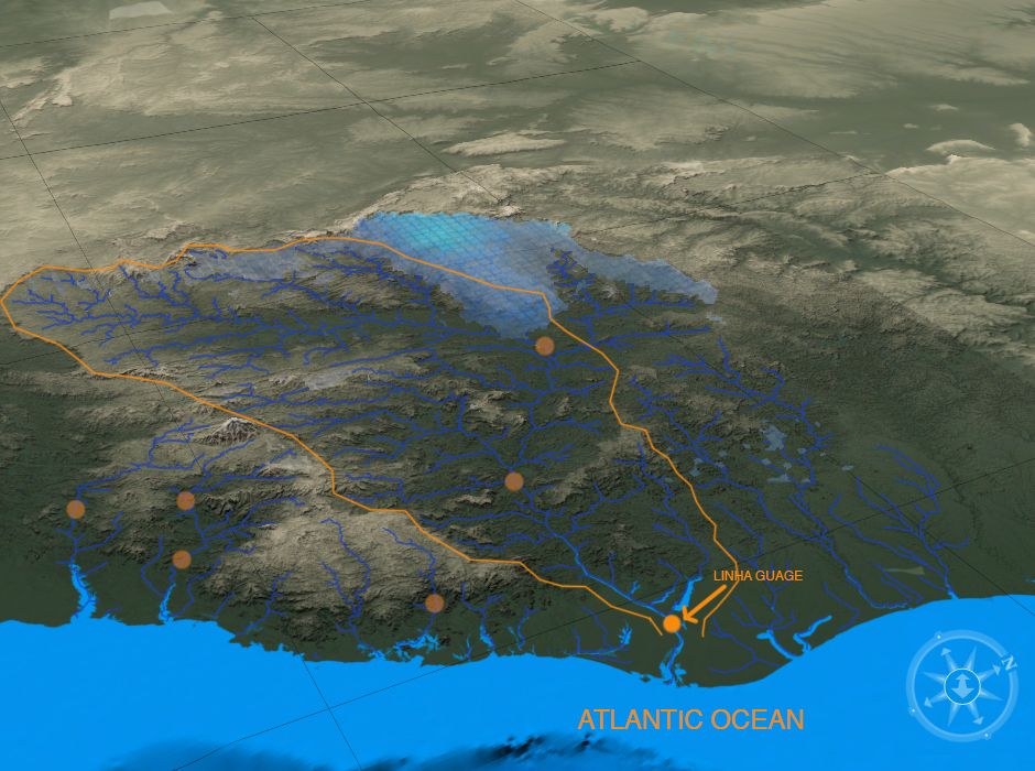
The watershed is a major river system within Espirito Santo (other rivers in the state are shown outside of the orange boundary line). The watershed drains into the Atlantic Ocean in southern Brazil (just north of the coastal state of Rio de Janeiro), affecting the ocean modeling work done off the coast. The World Bank funded research to ascertain whether development could be moved from Rio (a highly-developed state) to Espirito Santo (an untouched state in comparison) as the Espirito Santo government was concerned about the quality and quantity of water available to its residents.
Bruce used a popular subway map algorithm to look at the stream network of the watershed:
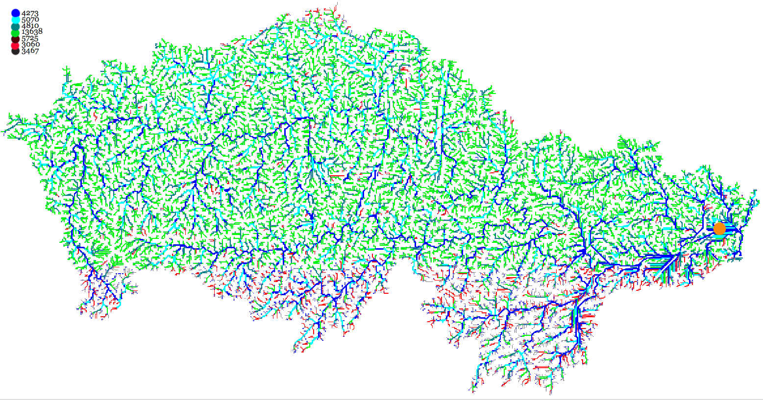
The streams were clustered by the amount of average flow in the channel (a count by network segment type, largest to smallest, appears in the upper-left corner).
The same algorithm was applied to look at potential changes to stream flow due to precipitation due to climate (or development) scenarios. In the example below, the number of streams increasing or decreasing in response to a change scenario are similar:
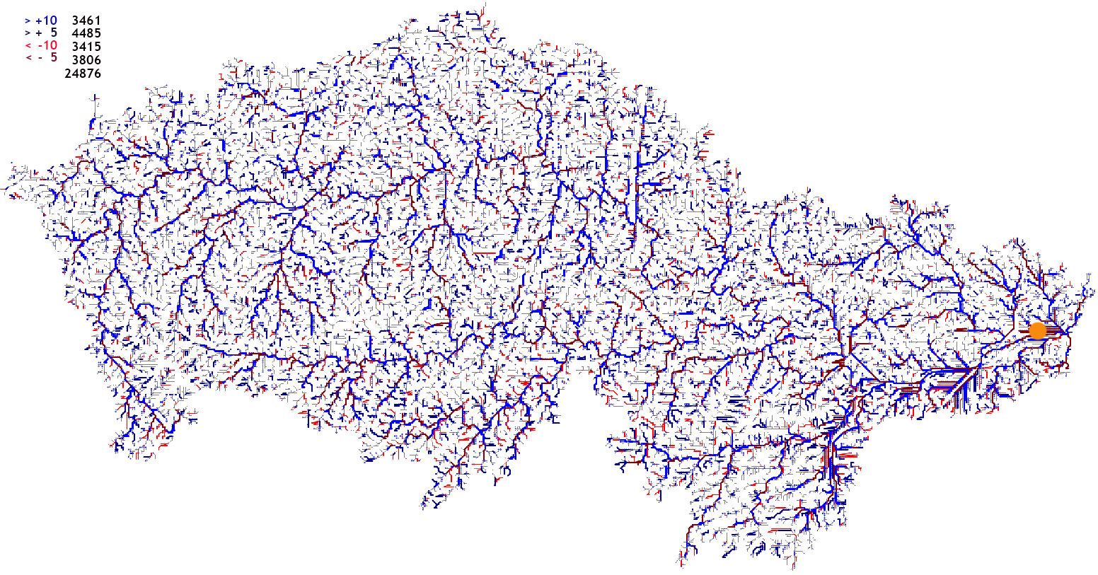
The legend in the upper left counts stream network segment changes (a segment is a stream channel between branches at both ends) and colors them by 10% or more increase, 5-10% increase, 10% or more decrease, 5-10% decrease and between -5 and 5% change.
The modelers then created their modeling application through a complex hydrological modeling process (using local methods and consulting from the UW) and Bruce obtained data for the observed gauge data, and seven different scenarios. P110/T0 is a scenario of ten percent more precipitation, P100/T1 is a scenario of a one-degree Celsius temperature increase, P100/T2 is a scenario of a two-degree Celsius temperature increase, P100/T3 is a scenario of a three-degree Celsius temperature increase, P90/T0 is a scenario of ten percent less precipitation, P80/T0 is a scenario of twenty percent less precipitation, and P80/T0 is a scenario of thirty percent less precipitation.
Students can use the legend in the lower-right to add or remove the scenarios from the visual analytics application. In the screenshot here, The P100/T0 scenario (no change to precipitation or temperature), Observed, and P70/T0 scenarios are active in the display:
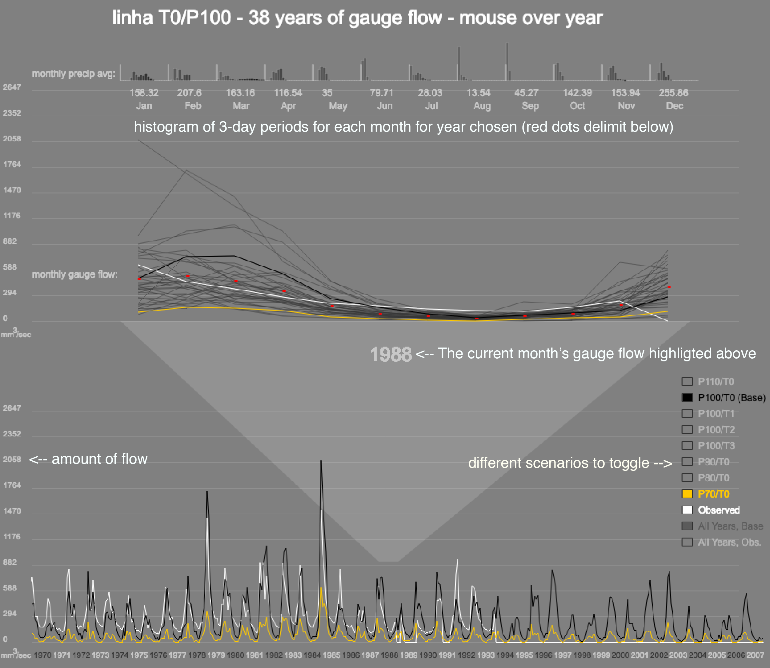
The outputs show three different sub-visualizations that can be used to perform an analysis visually (interaction is a key component of visual analytics). The top region shows the spread of precipitation for each three-day period in a histogram presentation (vertical bars show the relative amount of each 3-day period from left (close to none) to right (highest periods experienced)).
The middle region shows a monthly view of the three scenarios for 1988 among all other scenarios (keeping the white for observed, black for the base, and yellow-orange for the 3 degree temperature increase). Average values for all years in the base model are shown as red dots.
The bottom region highlights the differences between selected scenarios for all study years, where the model is applied retroactively to be compared with observed. Using retroactive approaches are popular, but have known concerns — for one, they don't necessarily capture behavior outside of the range expressed during the period. Climate changes for that region of Brazil are projected to be quite significant in upcoming years, so models will have to be updated any time behavior is experienced that differs from previous experience.
Issues with the retroactive modeling approach would be exacerbated by development changes within the study period, but the state had had very little development in the upstream areas.
Since the end of the World Bank's funded modeling period, additional methods based on emergent climate change modeling techniques have been applied.
Bruce then ran a whiteboard exercise whereby students worked through differences in visual processing systems of other beings:
and continued with a series of questions regarding technologies that help us see:
Students considered a visual analytics application for a watershed in the Brazilian state of Espirito Santo.
Bruce created the application to help a team at the University of Washington (UW), working with hydrologists in Brazil, visualize the outputs of water quantity modeling for the watershed seen here:
The watershed is a major river system within Espirito Santo (other rivers in the state are shown outside of the orange boundary line). The watershed drains into the Atlantic Ocean in southern Brazil (just north of the coastal state of Rio de Janeiro), affecting the ocean modeling work done off the coast. The World Bank funded research to ascertain whether development could be moved from Rio (a highly-developed state) to Espirito Santo (an untouched state in comparison) as the Espirito Santo government was concerned about the quality and quantity of water available to its residents.
Bruce used a popular subway map algorithm to look at the stream network of the watershed:
The streams were clustered by the amount of average flow in the channel (a count by network segment type, largest to smallest, appears in the upper-left corner).
The same algorithm was applied to look at potential changes to stream flow due to precipitation due to climate (or development) scenarios. In the example below, the number of streams increasing or decreasing in response to a change scenario are similar:
The legend in the upper left counts stream network segment changes (a segment is a stream channel between branches at both ends) and colors them by 10% or more increase, 5-10% increase, 10% or more decrease, 5-10% decrease and between -5 and 5% change.
The modelers then created their modeling application through a complex hydrological modeling process (using local methods and consulting from the UW) and Bruce obtained data for the observed gauge data, and seven different scenarios. P110/T0 is a scenario of ten percent more precipitation, P100/T1 is a scenario of a one-degree Celsius temperature increase, P100/T2 is a scenario of a two-degree Celsius temperature increase, P100/T3 is a scenario of a three-degree Celsius temperature increase, P90/T0 is a scenario of ten percent less precipitation, P80/T0 is a scenario of twenty percent less precipitation, and P80/T0 is a scenario of thirty percent less precipitation.
Students can use the legend in the lower-right to add or remove the scenarios from the visual analytics application. In the screenshot here, The P100/T0 scenario (no change to precipitation or temperature), Observed, and P70/T0 scenarios are active in the display:
The outputs show three different sub-visualizations that can be used to perform an analysis visually (interaction is a key component of visual analytics). The top region shows the spread of precipitation for each three-day period in a histogram presentation (vertical bars show the relative amount of each 3-day period from left (close to none) to right (highest periods experienced)).
The middle region shows a monthly view of the three scenarios for 1988 among all other scenarios (keeping the white for observed, black for the base, and yellow-orange for the 3 degree temperature increase). Average values for all years in the base model are shown as red dots.
The bottom region highlights the differences between selected scenarios for all study years, where the model is applied retroactively to be compared with observed. Using retroactive approaches are popular, but have known concerns — for one, they don't necessarily capture behavior outside of the range expressed during the period. Climate changes for that region of Brazil are projected to be quite significant in upcoming years, so models will have to be updated any time behavior is experienced that differs from previous experience.
Issues with the retroactive modeling approach would be exacerbated by development changes within the study period, but the state had had very little development in the upstream areas.
Since the end of the World Bank's funded modeling period, additional methods based on emergent climate change modeling techniques have been applied.
Bruce then ran a whiteboard exercise whereby students worked through differences in visual processing systems of other beings:
1. Honeybee
2. Bat
3. Eagle
4. Cat/Dog
5. Mole Rat
Bruce asked students what they would do differently if they were designing the human visual physiology from scratch
and continued with a series of questions regarding technologies that help us see:
1. What aspects of your visual system design would you be willing to outsource to technology?

2. How should such technologies be developed?

3. How should those technologies be distributed?

4. How much of your brain's sensory processing would you be willing to allocate to your visual
   processing in competition with your hearing, touching, smelling, and tasting processing?

5. What % of the time do you think your eyes deceive you based on a preconception you hold in
   memory from past experience (and what tech would you want to alert you to that potential)?