University of Rhode Island PODS Certificate

Class on March 6 2019

We started class with a JavaScript example (extended from the previous week) of how to plot an ASCII grid file with JavaScript, while using an image as the colormap based on the altitude of each location in Narragansett Bay. The HTML code can be saved in a basemap.html file:

<!DOCTYPE html>
<html lang="en">
  <head>
    <meta charset="utf-8">
    <title>Plot Bathymetry</title>
    <link rel="stylesheet" href="style.css">
  </head>
  <body>
    <canvas id="myCanvas" width="576" height="72" style="border:1px solid #d3d3d3;">
    	Your browser does not support HTML5 image-based color mapping.
    </canvas>
    <img id="colors" src="62Blb.png" style="visibility:hidden" /><br/>
    <input type="file" name="file" id="file"><br/><br/>
    <canvas id="plot" width="2500" height="2500"></canvas>
    <script src="script.js"></script>
  </body>
  <script>
	  var c = document.getElementById("myCanvas");
	  var context = c.getContext("2d");
	  var img = document.getElementById("colors");
	  alert('Choose the Browse button to select your .asc file for visualization.');
	  context.drawImage(img, 0, 0);
	  imgData = context.getImageData(0, 0, 576, 72); // get the 576x72 image 2D array
  </script>
</html>

while additional scripting code can be saved in a script.js file, as referenced in the HTML above:

  /* 
   * Get a color from the color map image based on plot value from bathymetry
   */
  function getColor(value) {
        color = [];
    
        if(value != undefined && value < 0) {
		value = value*-576/80;
		//below is how to access to your pixel details (stored in four integers)
		red=imgData.data[Math.floor(value)*4];
		green=imgData.data[Math.floor(value)*4+1];
		blue=imgData.data[Math.floor(value)*4+2];
		alpha=imgData.data[Math.floor(value)*4+3];
		color = [red,green,blue];   	
        } else {
		color = [0,0,0];
  	}
  	return color;
  }

  /* 
   * Plot the bathymetry by creating pixels for each row, column combination
   */
  function plot(data, ncols, row) {
        values = data.split(' ');
  	for(i=0; i<ncols; i++) {
	  var c = document.getElementById("plot");
	  var ctx = c.getContext("2d");
	  color = getColor(values[i]);
	  ctx.fillStyle = "rgba("+color[0]+","+color[1]+","+color[2]+",1)";
	  ctx.fillRect( i, row, 1, 1 );
	}
  }
  
  /* 
   * Read and plot the user's chosen .asc file
   */
  document.getElementById('file').onchange = function() {
	  var file = this.files[0];
	  var reader = new FileReader();
	  reader.onload = function(progressEvent){
	  //Read the lines into an array
	  var lines = this.result.split('\n');
	  var ncols = lines[0].split(' ');
	  ncols = ncols[1];
	  var nrows = lines[1].split(' ');
	  nrows = nrows[1];
	  document.getElementById('plot').width = ncols;
	  document.getElementById('plot').height = nrows;
	  var count=0;
	  for(var line = 6; line<lines.length; line++){
	    plot(lines[line], ncols, count);
	    count++;
	  }
	};
	reader.readAsText(file);
  };

The result appeared in the browser as:

Bruce then demonstrated how to use MAMP to import a data model and a data collection of Narragansett Bay buoy stations into the MAMP environment.

Students worked in teams to present the data on top of the base maps they created previously.

For example, a python notebook that plots Narragansett Bay buoy station data on the basemap. The notebook uses two Python libraries that are not installed initially during the Anaconda package manager software installation. They can be installed using the Anaconda commands:

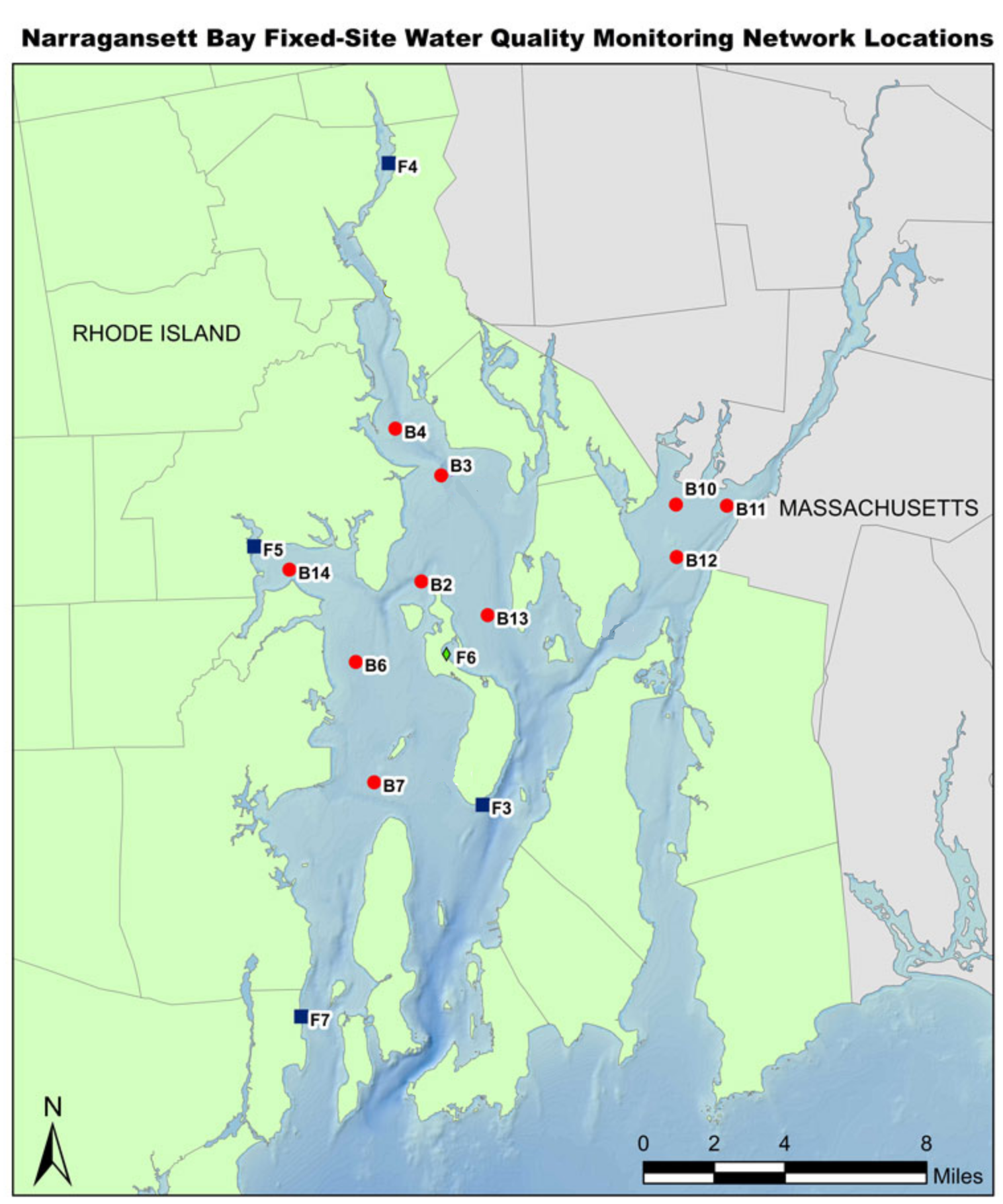
conda install netcdf4
conda install basemap-data-hires

The buoy information comes from two sources (merged together in the buoys.csv file). First, we use data from the Narragansett Bay Fixed-Site Water Quality Monitoring Network:

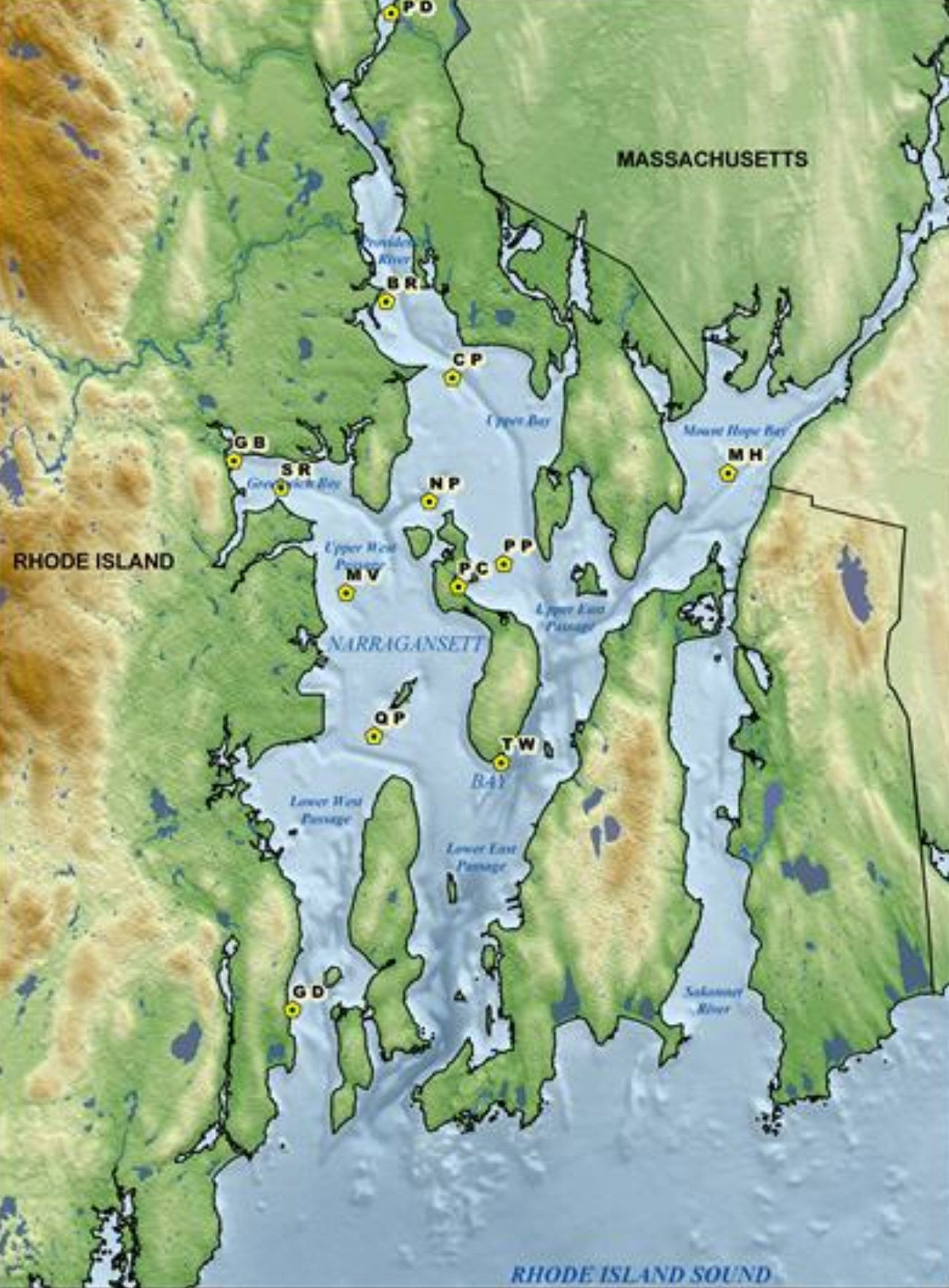
and second we add data from the National Atmospheric and Oceanographic Organization:

To process the comma-separated values (CSV) file, we used a Python package named Pandas in the second cell of the notebook. Pandas is very popular for reading and parsing scientific data:

# Use pandas to read in csv file
data_df = pd.read_csv('buoys.csv')

# Assign variables according to header line (i.e., first row)
lon = data_df['longitude']
lat = data_df['latitude']
w_temp = data_df['water_temp']

In the final cell of the notebook, we also converted the data columns we wanted to use in visualization to numpy arrays (to match the data format used for the underlying basemap):

lonnew = []
latnew = []

# Convert to NUMPY array.....VERY IMPORTANT
for i in range(0, len(lon)):
    lonnew.append(lon[i])
    latnew.append(lat[i])

x, y = m(lonnew, latnew)

And we added a scatter plot of the x (longitude) versus y (latitude) of the buoy locations:

plt.scatter(x, y, c='r', s=50, alpha=0.75, vmin=0, vmax=15)

and then used the x and y to place text representing a temperature value (in degrees Celsius) to the right of each buoy location:

for i in range(0, len(w_temp)):
    plt.text(x[i], y[i], str(w_temp[i]), color='w', size=15, horizontalalignment='left', 
             verticalalignment='center')

The matplotlib plotting library will render plot commands in the order they appear in the code (so we do the basemap first and then the scatter plots, and then the text). The plt.show() method identifies when we want the figure to be output to the notebook.

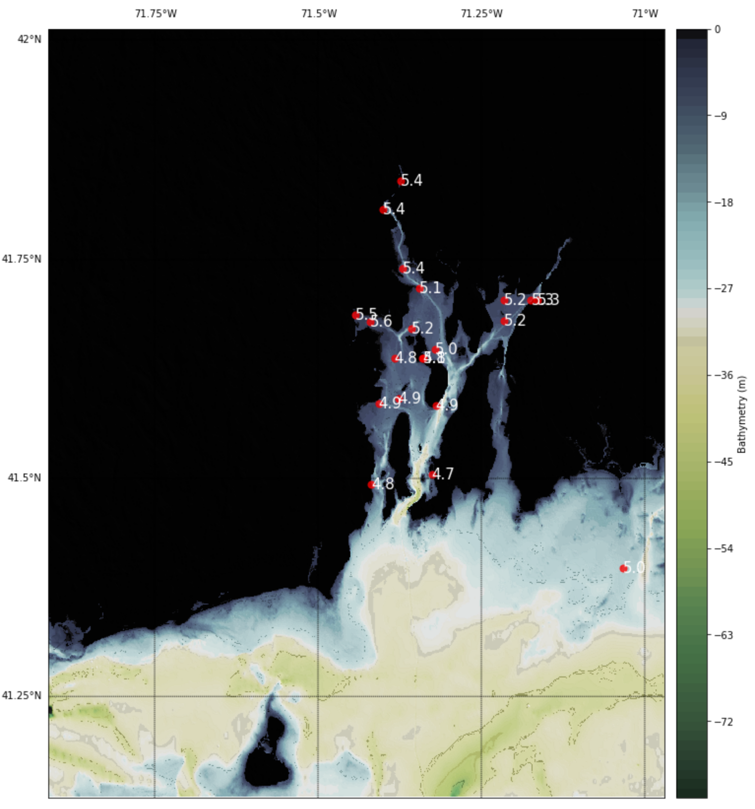
If all five cells run properly, the notebook generates a final image with the buoy information laid over the basemap created in class 2:

Bruce provided an assigned reading for homework in preparation for next class.