

Class on April 22 2019
Project 1 Presentations
We performed critiques for half of the students. As an example of a mid-term project, take a look at this student's project which is rendered here:
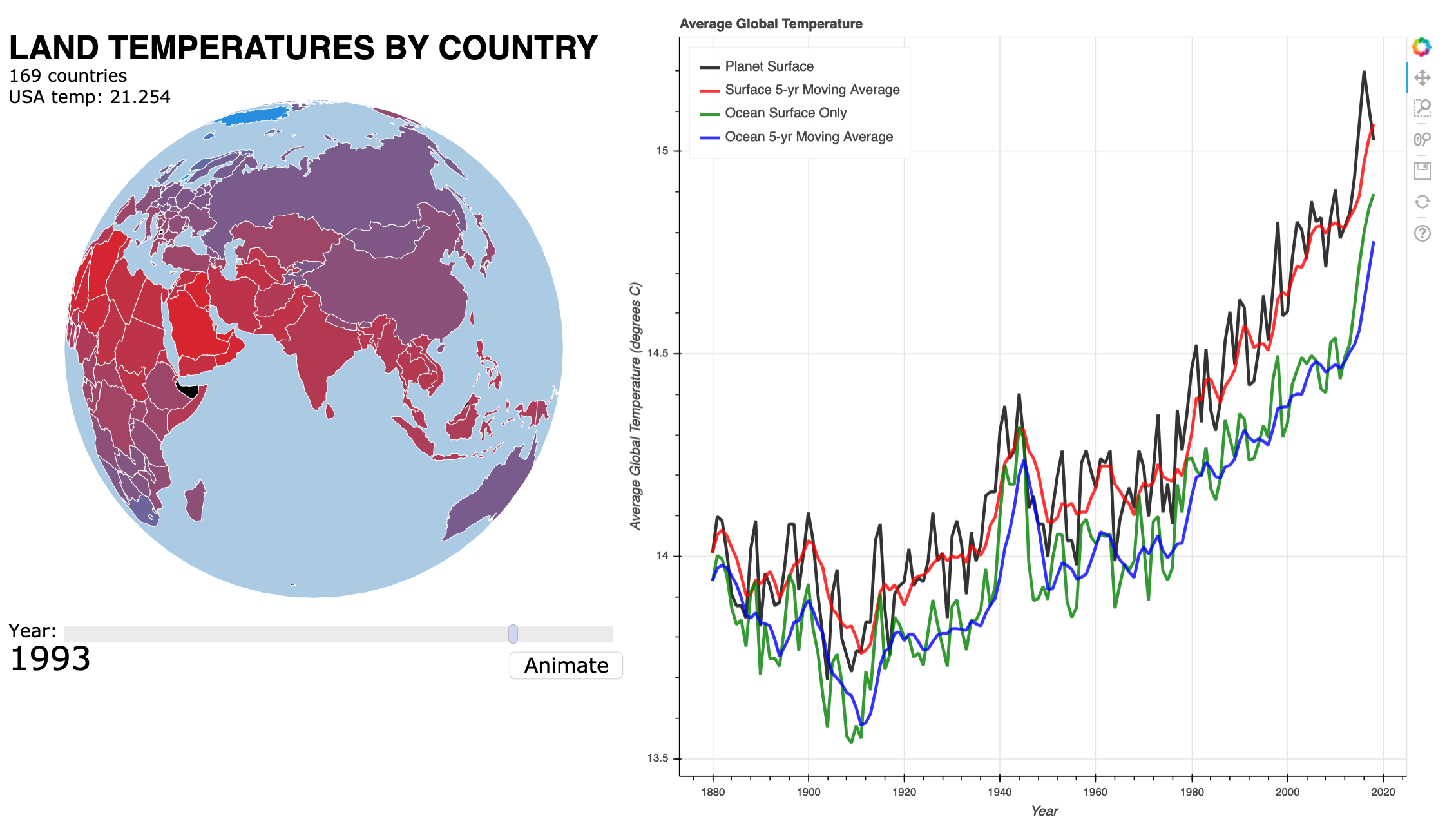
The left half was created as an extension of the D3 globe services provided in the April 8th class notes (second half of the page). The student found temperature data by country and injected it into a yearly representation on the globe using JavaScript:
A year selection slider lets her audience choose a year for visualization (and can rotate the globe by dragging side to side on any country), or she can run an animation of all the years by clicking on the Animate button. Clicking on the button fires an onclick handler that runs a JavaScript function:
The Bokeh cell that generates the plot has Python code:
The Bokeh package's output_file() method generates the temp-celcius.html HTML document.
We performed critiques for half of the students. As an example of a mid-term project, take a look at this student's project which is rendered here:
The left half was created as an extension of the D3 globe services provided in the April 8th class notes (second half of the page). The student found temperature data by country and injected it into a yearly representation on the globe using JavaScript:
	for(i=0;i<1000;i++) {
		if(tempById[i] != undefined) {
			  document.getElementById("country_"+i).style.fill =
			  "rgb(" + ((210*tempById[i]+1958)*1/43) + "," +
			           ((5903-tempById[i]*126)*1/43) + "," +
          		           ((9308-tempById[i]*210)*1/43) + ")";
		}
	}
The for() logic loops actively looking for all the country IDs between 0 and 999 (knowing that all the IDs are less than 1000). Each country is colored through the style fill attribute
using an ID attribute on the element that was established (named "countryXXX" where XXX is the country ID identified in the JSON and CSV data files).
A year selection slider lets her audience choose a year for visualization (and can rotate the globe by dragging side to side on any country), or she can run an animation of all the years by clicking on the Animate button. Clicking on the button fires an onclick handler that runs a JavaScript function:
	function animateData(showyear) {
		 updateData(showyear);
		 document.getElementById('current_year').innerHTML = showyear;
		 document.getElementById('myRange').value = showyear;
		 if(showyear < 2013) {
			  showyear++;
			  setTimeout(function(){ animateData(showyear+1); }, 500);
		 }
	}
The right half of the student's project is generated by Bokeh from within a Python notebook
using the temperature data students worked with in the March 27th class notes.
The Bokeh cell that generates the plot has Python code:
data_df = pd.read_csv('data/temperature-celsius.csv')

year8 = data_df['year']
surf = data_df['surface']
surf_mov = data_df['surf-mov']
ocean = data_df['ocean']
ocean_mov = data_df['ocean-mov']

plt = figure(plot_width=800, plot_height=800, title="Average Global Temperature")

plt.line(year8, surf, line_width=3, color='black',
         alpha=0.8, legend="Planet Surface")
plt.line(year8, surf_mov, line_width=3, color='red',
         alpha=0.8, legend="Surface 5-yr Moving Average")
plt.line(year8, ocean, line_width=3, color='green',
         alpha=0.8, legend="Ocean Surface Only")
plt.line(year8, ocean_mov, line_width=3, color='blue',
         alpha=0.8, legend="Ocean 5-yr Moving Average")

plt.xaxis.axis_label = 'Year'
plt.yaxis.axis_label = 'Average Global Temperature (degrees C)'

plt.legend.location = "top_left"
plt.legend.click_policy="hide"

output_file("data/temp-celcius.html", title="Average Global Temperature")
show(plt)
The Python relies on services from both the Pandas and Bokeh Python packages.
The Bokeh package's output_file() method generates the temp-celcius.html HTML document.