Book text is in a living document format, licensed under a Creative Commons Attribution-NonCommercial-NoDerivs 3.0 Unported License. In other words, you are free to share this work for non-commercial purposes as long as you don't create derivative works of this material, attribute me as the author, and keep this license notice intact. For more information about this Creative Commons license, please visit: http://CreativeCommons.org.

Chapter 7

systems simulation for understanding nature

We anticipate the state of the natural world to improve the quality of our own lives. The anticipation comes from expectations we make based on experiencing the natural world and it's various rhythms that occur over time. Those who invest the time to understand weather might anticipate a sunset if the joy of experiencing sunsets is something that moves them. Now that I've experienced the beauty of a blood-red harvest moon rising through the ocean, I've developed a more keen interest in the moon phase cycle come September and October each year. Those who get giddy over the annual flyover patterns of bird migration invest in considering a wide range of factors that affect the natural world. Some people coordinate their anticipation through a long list of facts and heuristics they maintain in their personal knowledge base. Others, like me, have found that systems simulations provide a more efficient mechanism for anticipating nature by more efficiently storing a model for rules generation than the long list method. In that case, even the list-items that do attach themselves seem less cumbersome to remember with a simulation at their base.

This chapter is the first of three chapters that provide representative case studies into the power of system simulations to provide understanding and insight. Simulations are often built for their power of prediction and decision-support. Let's focus on understanding and insight since those metrics offer us the opportunity to explore without having specific reasons ahead of time. We can build, run, and investigate simulations and see where our thought processes turn before they turn to known benefits. Only afterwards, once we've had our own independent thoughts and experiences, can we consider the experts' knowledgeable use of the simulation. At that point, I ask myself whether those considerations are natural ramifications of my own thoughts or if they are exceptions. I invest time into understanding the exceptions for they are most likely to seem foreign to me most often. Those that are natural tend to be remembered much easier than those that seem foreign. And, of course, I don't shortchange my right and opportunity to challenge the exceptions — even though those challenges are often unfounded by the time I understand better what the experts already understand. The process itself seems meaningful.

Let's start with the mother of natural systems simulations. Meteorologists have made great strides in predicting weather during my lifetime. As a result, meteorology is a great case study in the potential of simulation for understanding nature. Weather is complex (and fickle) friend of ours as we find conditions changing over time and place in ways that force us to anticipate future weather based on past experience. The collective knowledge of all meteorologists is a brain trust that allows us to inject weather consideration into our daily lives — which has also been great for starting up conversations with strangers we might not start up otherwise. Such conversations often feel more meaningful when I am in unfamiliar surroundings.

As we look at the dynamic range of natural conditions on the planet, we find that some areas are harder to predict weather for than others. There are natural convergence zones where weather in higher latitudes mixes with weather in lower latitudes and creates larger gradients of behavior over smaller distances. We have coastal zones where relevant weather data is harder to acquire as no one lives on the ocean consistently to report the data — and our ocean-based sensors confront rough conditions to keep reporting reliably. We have regions where cloudy conditions are much more prevalent — limiting our ability to gather highly relevant data by remote sensing satellites way up in orbit. And then, of course, we have more reliably uniform weather regions on the planet where weather forecasting is significantly simpler — although longer-term climate change moves those regions ever so slightly from year to year.

Weather is a significant driver (also called a forcing agent) in modeling other natural systems we encounter on our planet — and thus critical for many natural system simulations. As a result, we have put a lot of time and effort (and research money) into simulating weather systems in order to understand and better predict weather in the future. Meteorologists have become recognizable community figures as they have learned to communicate model outputs to others.

One interesting follow-on simulation we can use as a case study looks at the effect weather has had when investigating water movement on the planet: How does water move from atmosphere to land to water network to ocean to atmosphere again? The behavior of water as it passes by us in streams and rivers might matter most when flooding is involved. But, the behavior of water is a fascinating place to invest one's thought and insight-generation powers. We might take water for granted thanks to nature's competent stewardship on a day-to-day basis. Or, we might live in a community that can't afford to be as cavalier since water issues affect the community more noticeably more often. We can build compassion for those communities that have struggled with water issues by growing our understanding and insight of water through interaction with visual simulations.

If we use the often-used word watershed as the geographical area where water exists and yet moves downhill to the same eventual exit locale, we can then say that the hydrology modeling effort to simulate water movement is a key component of all watershed simulation — simulation that looks at any behavior of man-made or other process within the bounds of a geographical watershed.

My first exposure to natural systems simulation started with hydrology modeling as an impressive cadre of natural systems simulation experts introduced me to the hydrology component of watershed simulation. Although those experts had each come to prominence by focusing on a specific natural domain regardless of watershed geography, the university was asking them to coordinate their research on behalf of the greater local watershed known as the Puget Sound region, for a better integrated understanding of residents' actions on the health of systems that provide fresh water inputs to the sound — the body of water that dominates the local economy and recreation activities.

As it turns out, hydrology modeling is often one of the easier components to simulate in a watershed domain. In many situations on our planet, hydrology is straightforward and floods, drinking water supply, and minimal water levels to support life year-round can be predicted to a necessary precision quite consistently if the weather forecast is accurate — in other words, the hydrology is mainly a result of weather precipitation, temperature, wind, and evaporation (each of which is predicted in a weather forecast). It's harder to model the interaction of that water with plants and animals (including us humans). Sometimes the modeling effort is more difficult due to convergence zone weather issues and complex terrain.

The Puget Sound area is unique in that it sits between two mountain ranges that amass water content as snow pack for much of the year. The mountains are high in elevation and include dramatic slopes as the elevation lowers from mountaintop to sea level over a relatively short distance (way shorter than the Mississippi-Missouri waterway, for example). The temperature at the mountaintops can be quite different from the temperature at sea level and the geographical spread of the temperature gradient can vary significantly from day to day. Rain at sea level does not mean rain at the mountaintop and sun at sea level does not mean sun at the mountaintop. Wind effects add complexity. The diversity of behavior over the course of a year provides a complex environment for simulating water flow — and water flow in times of potential flood levels is very valuable to those living near river systems.

We take a look at the hydrology-modeling component of a watershed simulation in this chapter. We compare a simple model that is effective for a stable environment to a complex model that is effective for a dynamic environment. It's an ideal case study for learning how to focus on simulation development by differentiating inputs, processes, and outputs — since the community of hydrology experts has evolved their identification and conventional naming significantly over time. And, of course, each input, process, or output can help us practice our simulaton life skills as we have likely interacted with each input, process, and output often in our lives and can readily conjure up each in our imagination on demand.

There are many hydrology modeling software toolkits available to support maintaining a simulation. A search on 'USGS hydrology software' brings up representative lists based on categories of focus such as: General Use, Water Quality and Chemistry, Groundwater, and Surface Water. A description of a surface water toolkit named HSPF (for Hydrology Simulation Program Fortran — fortran being the programming language used for ready implementation) is representative of how fit for purpose is identified for others to consider:

HSPF simulates for extended periods of time the hydrologic, and associated water quality, processes on pervious and impervious land surfaces and in streams and well-mixed impoundments.

Each software toolkit is optimized to consider specific inputs, simulate specific processes, and provide specific outputs. Let's consider the inputs required of a simulation toolkit for a basic watershed condition (relative uniform weather and limited elevation change):

1. Rainfall is a primary input — something most of us would anticipate as being critical to hydrology simulation.
2. Elevation is a primary input as it defines the terrain over which rain will fall — most of us can easily envision how gravity pulls water downhill faster over a steep elevation change than a gradual one.
3. Soil moisture is often a primary input as it defines whether more water can be absorbed by soil within the watershed or whether the water will run downhill without the opportunity to be caught.

Even soil moisture can become irrelevant to the model should the ground be so impervious (for example when covered with bedrock at the surface) that soil moisture becomes immaterial. Most of us can imagine a watershed within a rocky mountain range where all the water falls on rock and moves downhill to a lake at the bottom of the elevation. Our simulation model in those situations is likely going to be as good as the weather forecast. If we can predict the rainfall (and the evaporation of water back to the atmosphere on sunnier days), and the terrain doesn't change by some unlikely geological event (a mass wasting event like a rock slide or interruption by volcanic activity), we don't need much software support to create a solid simulation of water behavior in that watershed.

The processes involved in that simplified environment include moving rainfall from the atmosphere to the land area that drains to the lake, moving water back to the atmosphere through evaporation, and moving water downhill from higher elevations according to the elevation profiles along the way. The output is a lake volume that consistently can be evaluated as a lake depth and a shoreline detail.

Starting from simple conditions and building upon them is a reasonable approach when wanting to build a stronger skill at simulating nature to support a simulaton life. By proceeding in that fashion, we gain insights and understanding at a comfortable rate and a comfortable rate can maintain our motivation. In the case of hydrology simulation, each complication we add likely interacts with most of what we have already considered previously. In fact, we'll make our soil input more complicated by chapter's end. For now, let's add another popular complicating factor to our simulation inputs:

4. Vegetation is often a primary input when the watershed upon which rain falls is filled with plant life that uses the water for life process — most of us can envision plants taking up water through its roots to support life processes within the plant.

The vegetation adds significant complexity to our simulation. The vegetation is dependent on the soil for its ability to live in that location. The vegetation is dependent on access to sunlight that is varied based on elevation and the direction of slope. And, of course, the vegetation is dependent on the rainfall for it's ability to stay alive. There are interactions among vegetation and all other inputs as soon as we add vegetation as an input to the simulation. The complexity behavior between soil moisture and vegetation is partially driven by root depth and partially driven by the water requirements of the vegetation. Some plants take up a lot more water than others. Soil that is saturated with plant roots behaves very different from soil that is porous but deeper than any root depth.

Adding vegetation as an input also means we can benefit from simulating the use of water by the plants. New processes help us become more precise in our simulation: plant transpiration moves water through a plant and evaporates water from aerial parts — especially from leaves but also from stems and flowers; plant photosynthesis uses water to produce sugars from sunlight; plant respiration burns sugars for energy when sunlight is not providing input to photosynthesis. Thankfully, the plant transpiration is a dominant process compared to photosynthesis and transpiration and we can add plant transpiration to overall evaporation of water from the watershed surface to create a single simulated process called evapotranspiration.

These vegetation effects to our hydrology simulation can vary significantly by time of year if the watershed experiences dramatic seasons. Plants don't take up water in winter if they are a species that goes dormant, for example. Some plants lose their leaves in preparation for winter. The effects of fire can dramatically affect the vegetation inputs being simulated. It's powerful to dwell on the effects life has on the behavior of water. Plants are just the beginning as of course animals, and particularly us humans, use water in life processes as well. Animals are not as limited by watershed boundaries and can move water from one watershed to another in the course of daily living.

With the addition of vegetation, we are already at a level of complexity in which we can continue to have insights and develop deeper understanding through simulating hydrology. In many cases, the effects are subtle but we as humans have the opportunity to explore the subtle effects, as the watershed we experience is the sum total of all effects and nothing else. If we plant a tree, we change the hydrology in the watershed to some degree. If we plant 100,000 trees as has been happening in some Scottish watersheds, we can change the watershed significantly. If we change the soil within the watershed, we change the opportunity plants have to thrive. Or, on the flip side, we increase the chances they won't. Clear-cutting a forest has been a much more recent change to the hydrology of a watershed than planting the same number of trees. Simulation tools have taught many forest managers a reasonable approach to managing tree harvest and replanting.

Let's add another complicating simulation input that isn't present in many watersheds but which can have a dominant effect when it is:

5. Snowpack forms from layers of snow that accumulate in geographic regions and high altitudes where the climate includes cold weather for extended periods during the year.

The snowpack grows as a season gets colder and shrinks when a season gets warmer (0 degrees Celsius being a reasonable starting point for expecting growing versus shrinking). A snowpack can accumulate tremendous amounts of water and keep that water from heading downhill for significant periods of time. The snowpack usually happens most where the potential energy of water is at its highest (where the momentum for downhill movement is greatest). We can imagine a watershed without soil and without vegetation that would be affected greatly by snowpack. Antarctica and Greenland are two large geographical regions that have been in the news often for their dominant effects of snowpack within their watersheds. As we add soil and vegetation to the model, we see how their effects are dwarfed by snowpack that prohibits water from reaching their contribution to the simulation.

Snowpack is so dominant in watersheds that accumulate huge volumes that specialized hydrology modeling software toolkits have been developed specifically for such watershed simulation. The DHSVM toolkit I used in the Puget Sound area is such a toolkit that considers snowpack along with all other inputs of significance within those watersheds. Let's consider all the relevant inputs of a significant snowpack watershed for simulating it to foster understanding and insight. Our list grows from the five already mentioned:

6. Wind becomes important as an input because snowpack interacts with wind to increase evaporation across the snowpack — the greater the wind, the increase in evaporation. Wind increases evaporation in places besides those covered in snowpack as well.
7. Air temperature becomes important as an input because snowpack melts faster for each additional degree in temperature as the air temperature increases well beyond the freezing temperature of water.
8. Shading becomes important as shade cools regions that can maintain snowpack more easily as a result. As snowpack changes the surface elevation away from the basic elevation input, shading changes as well.
9. Snow state becomes important as different snow types have different properties just as soil types have different properties.

We can also start to differentiate our previous inputs into more specific inputs. The soil input can be decomposed to include separate inputs as to the soil type, soil depth, and soil state — the latter as one that most readily changes throughout the simulation. The vegetation can include separate inputs as to vegetation type, root depth, and vegetation state — the latter as one that most readily changes throughout the simulation. Even the precipitation can be decomposed into amount and type (light, moderate, heavy, sleet, hail, snow).

To allow us to simplify our inputs in the aggregate and still be able to present outputs in a realistic manner, we add one last input to our model:

10. The stream channel input is a network of all the channels within the watershed that carry surface water downhill — we know these channels as streams and rivers — organized into a network of segments mapped to location and connectivity.

The stream channel is an observed phenomenon and so needs to be authentic to map the outputs of the simulation to actual objects that can be evaluated. Of course, if all the other inputs were perfect and of necessary resolution, the stream channel would be a pure output of the simulation (the elevation model would suggest where those streams should be). The cost of maintaining such a high-level of resolution in the simulation is more often not justified since the probability of additional insight is not enough to justify it. And so, the simulation must map its view of the world to water in the channel — something it does quite well, thankfully, once the stream channel input is made available.

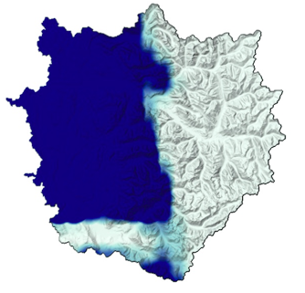
Existing hydrology simulation toolkits use a numerical format for inputs. Inputs are organized with awareness as to geographical location of each input. There are a variety of ways to map the inputs to geographical locations and each has some benefit to the simulation. Some mappings are better than others depending on the aspects of simulation that are being emphasized. The nature of inputs though is that each input can be investigated independently through interactive visual artifacts such as images. Here's two elevation inputs shown as images:

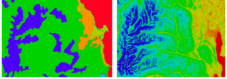
The left image represents a situation where elevation change is gradual and elevation is quite flat in most places. The right represents a situation where elevation change is rapid in places and elevation is quite sloped overall — blue is the highest elevation and red is the lowest. One insight to be gained through experience with hydrological simulations is that the complexity for simulating the hydrology in the left situation can be a lot simpler than the right situation for getting the same level of correlation with the physical world — the closeness of the simulated volume of water in each channel to the actual.

Each input can be explored through an image representation of the numerical inputs to the simulation tool. Inputs can be presented individually or together as layers:

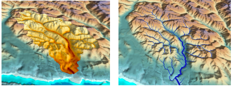
The left image shows the soil depth input within a watershed while the right image combines the stream channel network input as a blue presentation on top of the elevation input that is colored and shaded to suggest height in relief.

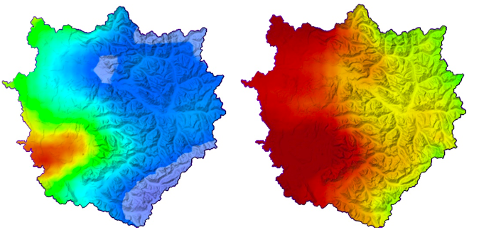
Each input to a hydrology simulation has its own natural temporal rhythm — the time period over which values tend to change. The elevation input is unique in that it is usually considered fixed throughout the simulation period — unless it is part of a scenario looking at elevation change for some simulated event that would change elevation. Soil depth, vegetation type, and soil type are examples of inputs that change slowly in a simulation. Soil moisture, precipitation, and wind are examples of inputs that change more rapidly — rapidly enough that the simulation keeps changing them continuously to move the simulation forward through time. When an input changes often through a shorter time rhythm of change, the input makes a prime candidate for animation to visually explore its input to the simulation. Here are a few examples.

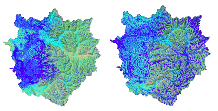
Air temperature animations show the change of air temperature over time. Blue color below is cooler than the red temperature. The warming trend between the left and right provides detail when animated over short time increments. Animations that cover a longer time period show patterns of how the air mass above a watershed cools and warms near the surface. Our brain's ability to pick out patterns provides insight into the nature of the temperature change.

Precipitation animations show patterns of rainfall over the same period of time. Our brains can explore the relationship between precipitation and air temperature when both are provided over the same time period. In this case, heavy rainfall is falling on the western half of the watershed with a very small transition zone to the dry half of the watershed to the east.

We can explore one of the more intricate inputs, soil moisture, through visualizing soil moisture animation over time. Soil moisture levels change across the watershed as the simulation runs. The mid-blue color below represents soil that has been saturated by moisture. Other colors represent percents of saturation that are less than 100%. In this case saturation moves from west to east, which is not surprising given that precipitation is moving from west to east as well.

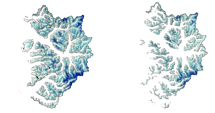
Snow pack animation provides insight into the effect of other inputs and processes on the amount of snow covering the terrain. Warm temperatures, rainfall, wind, and other inputs all affect the snow pack and an animation of snowpack simulates the rate of change over time. The dark blue color represents areas within the watershed with the most snow pack. Lighter colors represent values of less snow pack. White areas contain no snow pack. White areas increase as overall snow pack reduces over time.

Each input to the simulation is involved in at least once dynamic process that determines the flow of water. If the input were not involved in the computation of water movement, it wouldn't be directly relevant to the simulation. Some processes include many input types while others include just two or a few. The design of the simulation takes into account the relevance of each input to the authenticity of the result of computations. Some inputs may have an impact that is so small that the designers consider it immaterial for the typical range of system behavior seen in the physical world. Computation time reduces when inputs can be removed from being involved in a process. From that point of view, we can consider some of the processes often included in hydrology models and consider the impact of each input involved.

Gravity plays a dominant role in hydrology. Water moves downhill consistently in response to gravity as a force. Friction of water as it moves against and over surfaces slows the rate at which water moves. Different soils have different grain sizes. The smallest grains don't let water through once fully saturated. The largest grains let water through with least friction thanks to the open spaces available between grains. Other soil types vary from predominantly smaller grains to predominantly larger grains. Some are a complete hodge-podge of small and large grains all within a small volume. As a purely physical process, gravity moves water through its environment in predictable ways. Digital elevation inputs, soil inputs, vegetation inputs, and channel inputs all contribute to the computation of water movement due to the physical force of gravity. The simulation of the force of gravity plays a dominant part of predicting hydrology behavior in many environments. Other environments include relevant chemical and biological forces.

Evaporation plays a significant role in hydrology. Water returns to a vapor state from a liquid state over time in many hydrological environments. Without replenishing evaporated water through new precipitation or other phenomena that turn water vapor back into liquid, a watershed dries out over time through the evaporation process. The surface area of water available for evaporation is derived from the soil, vegetation, and channel inputs. The rate of evaporation is derived from temperature and wind inputs. A hydrology simulation computes the movement of water back into the air as a contribution to overall hydrology movement — a contribution that works against the force of gravity more than along with it.

Saturation plays a significant role in hydrology. When soil gets saturated with water, water can move over the soil instead of being drawn into it by gravity and other forces. When plants get saturated with enough water for their biological needs, they no longer need to take water out of the soil. The specifics of the soils and vegetation inputs to the hydrological model affect the simulation of water movement. Once a soil is saturated, soil type becomes less significant from a water run-off perspective. Water begins to run downhill much faster without the effects of soil and vegetation damping the movement.

Other processes vary widely depending on the characteristics of the watershed. Urban watersheds, or those that provide drinking water for urban watersheds, can be dramatically affected by human actions. Dams can change the movement of water downhill by creating reservoirs that catch the water without letting it progress. Pipes and culverts can redirect water. Pumps can drive water uphill against the natural pull of gravity. An urban hydrology simulation often benefits from the expertise of a civil engineer who studies the behavior of water in man-made environments. An urban behaviorist can help when simulating the draw human beings make of water reservoirs over time. A hydrology simulation can get significantly more complex when human behavior and man-made objects are active in the watershed. The outputs from one time step's worth of computation include parts of the input to the next time step's worth. As a result, the inputs and outputs available for investigating a hydrology simulation as it runs are tightly coupled and the artifacts that the simulation make available for insight and understanding are often similar enough to benefit from similar perception and cognition processes. A soil moisture animation artifact includes a view of soil moisture at each time step the simulation creates a discrete computation. The snow pack artifact includes a view of snow pack at each time step the simulation creates a discrete computation. The channel volume artifact includes a view of water volume in each channel for each time step in the simulation.

With enough artifacts providing changing views of key components to the hydrological simulation process, we have a wide variety of mental responses that can occur. Each mental process can be highly unique to each individual. As a result, a rich discussion can come from groups of people who gain access to the simulation with the goal of gaining insight and understanding.